LTspice Tutorial: Part 2
So we have learned how to enter a schematic in LTspice®. This LTspice tutorial will explain how to modify the circuit and apply some different signals to it.
To save you constructing a new schematic, download this file: 2nd order Butterworth low pass filter. The circuit is shown in Figure 1
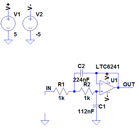
Figure 1
Note the voltage source is missing. To test the frequency response of the filter we could apply a sinewave input to the circuit and measure the amplitude of the output, then change the frequency of the sinewave and repeat the process. Or we could apply an ac sweep to the input and get a plot in the frequency domain instead of the time domain.
To add a generic voltage source go to 'Add Component' by clicking on the symbol and this should bring up the menu as shown in Figure 2
To add a generic voltage source go to 'Add Component' by clicking on the
symbol and this should bring up the menu as shown in Figure 2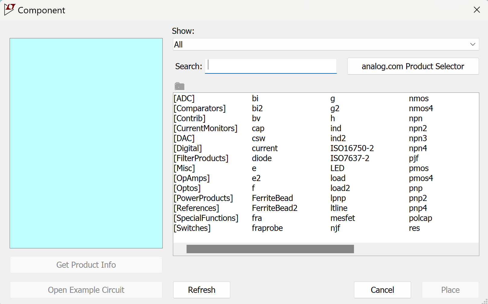
Figure 2
Scroll to the far right and add a 'voltage' and place it in the circuit.
To implement an ac sweep, right click over the voltage source and select Advanced to display the following:
To implement an ac sweep, right click over the voltage source and select Advanced to display the following:
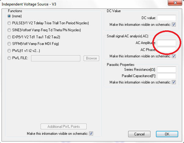
Figure 3
Keeping the Function selections as 'None' enter a voltage in the Small Signal AC analysis box. Enter an amplitude of 1V then click OK.
We now need to configure the simulator to perform the ac sweep.
In the schematic editor, click on Simulate -> Edit Simulation cmd then click on the AC Analysis tab. Enter the parameters as shown in Figure 4
We now need to configure the simulator to perform the ac sweep.
In the schematic editor, click on Simulate -> Edit Simulation cmd then click on the AC Analysis tab. Enter the parameters as shown in Figure 4
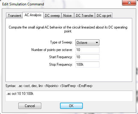
Figure 4
This sets the number of steps to be displayed per octave, with a start frequency at 10Hz and a stop frequency of 100kHz. Click OK and put the simulation statement anywhere on the schematic. The final circuit is shown in Figure 5
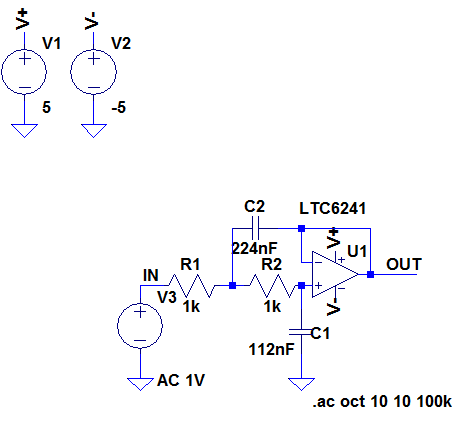
Figure 5
Save the file.
Clicking on the Run/Pause symbol will run the simulation. Probing the OUT node will plot the frequency response of the filter, clearly showing roll off above 1kHz. The phase response of the output with respect to the ac signal source is also plotted on the right hand y-axis.
If we want to magnify a certain area of the plot, move the crosshairs to the desired part of the plot, left click the mouse and, holding it down, drag it over the area to be magnified. The plot will then zoom into that area. The coordinates of the crosshairs are shown in the bottom left hand corner of the screen and when a box is selected, these coordinates show the differential values of the box. Since this example is plotted in the frequency domain, the x-axis displays frequency. If the x-axis shows the time domain, the coordinates show time and when a box is selected the coordinates show differential time and frequency.
Hitting the <F9> key undoes this action.
If you want to zoom in or out when in the schematic window, use the Zoom In and Zoom Out symbols on the menu bar. Alternatively the jog wheel on your mouse performs the same function. Holding down the left mouse button and moving it over the schematic allows you to pan over the circuit.
Hitting the space bar auto-sizes the schematic window.
The x-axis and y-axis settings can be changed by moving the crosshairs over the desired axis and left clicking the mouse.
To check the roll off characteristics of the filter, we need to display the cursors. Move the mouse to the 'Vout' logo at the top of the plot pane and right click. This brings up a menu to enable us to select between 1 cursor or 2. Selecting a single cursor results in Figure 6.
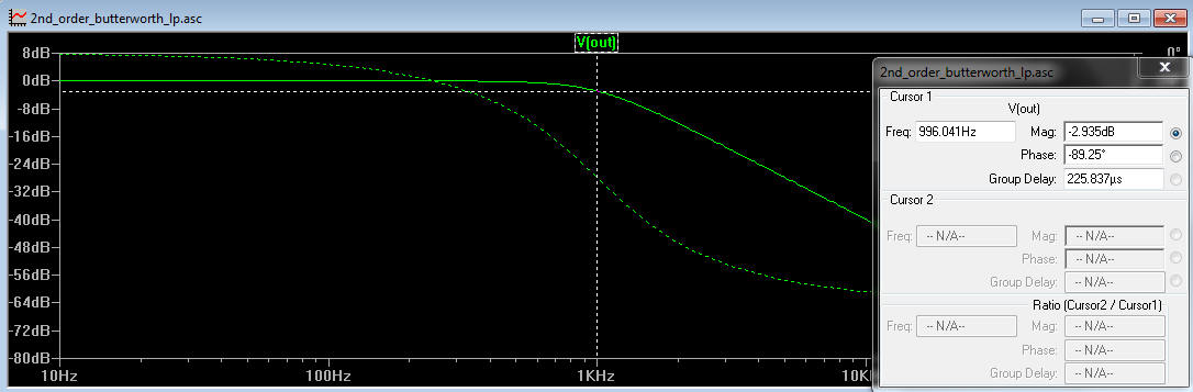
Figure 6
(the shortcut for displaying the single cursor is to left click on the waveform icon V(out)). To select 2 cursors, double click on the Vout icon.
Moving the crosshairs over the cursor and left clicking the mouse enables us to move the cursor and measure the magnitude and phase response of the circuit in the results box. Closing the results box removes the cursors. If 2 cursors are selected differential voltages and phases can be displayed.
We are now going to change the input signal from an ac sweep to a piecewise linear waveform. A piecewise linear voltage source consists of a series of voltages specified at certain instances in time with a linear change in voltage between them.
Firstly, delete the Simulation command (.ac OCT 10 10 100k)
Right click over the input voltage source to bring up the parameters dialogue box. Delete the ac amplitude and change the function button from (none) to PWL (piecewise linear).
The setting box should look like Figure 7
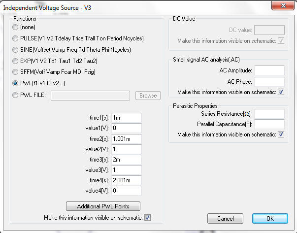
Figure 7
The waveform above starts at 0V, stays at 0V until 1m after which it rises to 1V in 0.001ms. It stays at 1V until 2ms, then falls to 0V in 0.001ms.
In the schematic editors, click on Simulate -> Configure Analysis and click on the Transient tab. Set the transient analysis to have a stop time of 5ms and click OK.
Clicking the Run/Pause symbol brings up the plot pane as shown in Figure 8
In the schematic editors, click on Simulate -> Configure Analysis and click on the Transient tab. Set the transient analysis to have a stop time of 5ms and click OK.
Clicking the Run/Pause symbol brings up the plot pane as shown in Figure 8
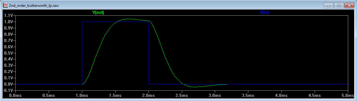
Figure 8
Probing the IN and OUT nodes shows that although the Butterworth filter has excellent pass band performance, it is a poor filter to use if trying to maintain the shape of a pulse.
Note: If the PWL input starts at a non zero voltage, the Y axis of the plot pane will start at a non zero voltage.
Run this simulation:
LT1761 with Vin starting at 3.5V
The input to this 3v3 linear regulator starts at 3.5V and ramps to 5V. Plot the output voltage. The Y axis of the plot pane starts at 3.2V, not 0V
In the simulation below, the PWL input voltage has been changed to start at 0V instead of 3.5V. Now the Y axis of the plot pane starts at 0V:
LT1761 with Vin starting at 0V
Want to know more?
Please see LTspice Tutorial: Part 3
If you want to learn about noise measurements see this article: Op Amp Noise Analysis
LTspice is a registered trademark of Analog Devices Inc
Sitemap: www.simonbramble.co.uk/sitemap
© Copyright Simon Bramble